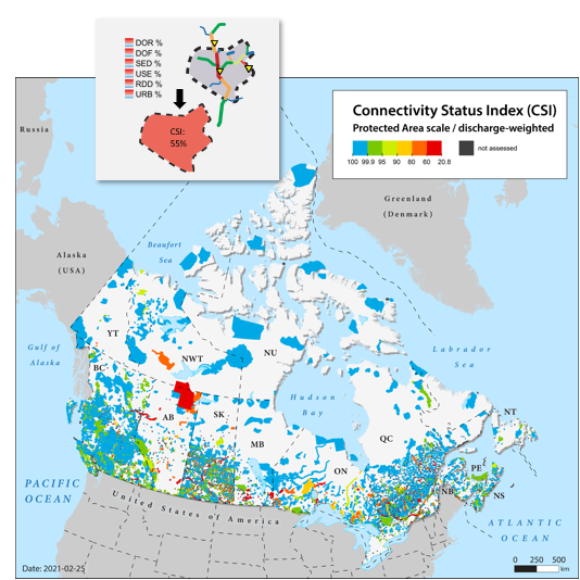
Using the CSI to assess the connectivity status of protected areas in Canada
Using the CSI to assess the connectivity status of protected areas in Canada
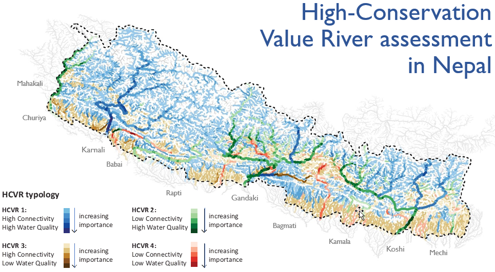
Classification of high-conservation value rivers using the FFR approach.
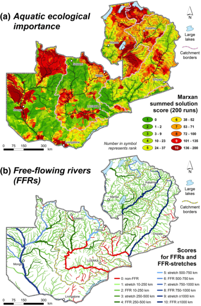
Identification of water resource protection areas using the FFR approach
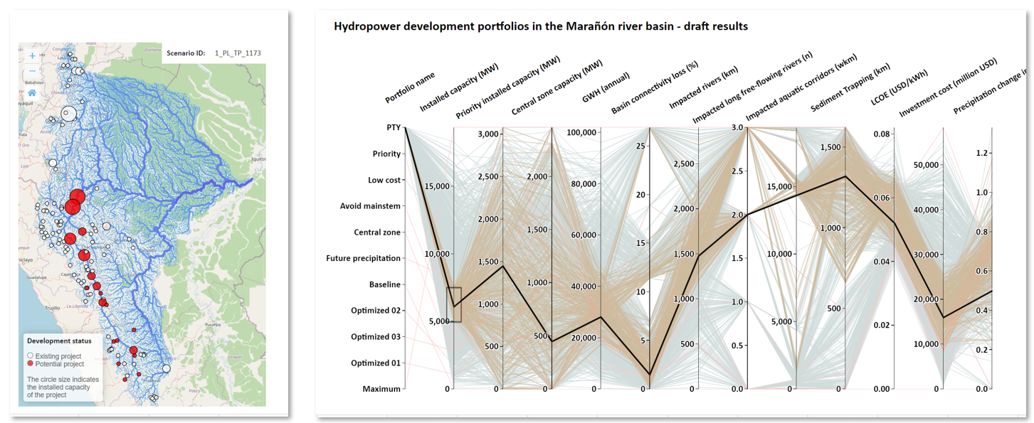
Using the CSI and the FFR status in Hydropower planning in Peru
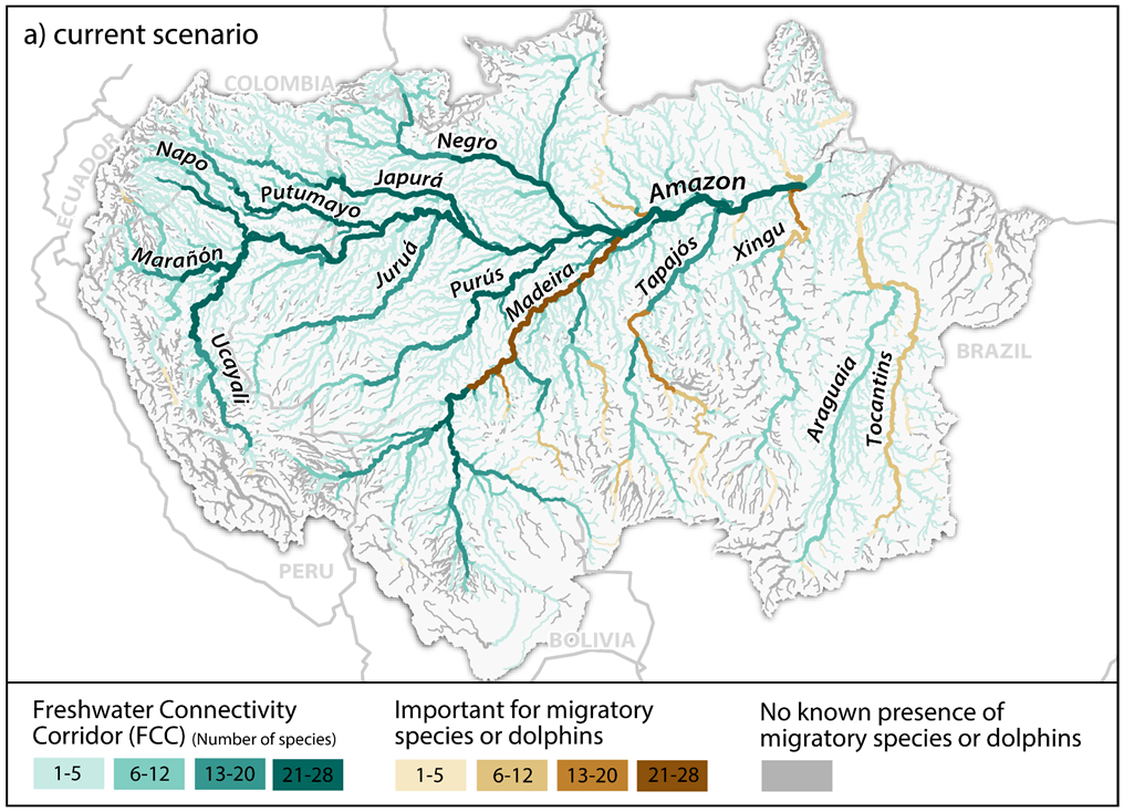
Freshwater connectivity corridors in the Amazon River basin
| Step | Instruction |
|---|---|
| 1 | Identify and analyze different road layers and create a list. |
| 2 | Choose the most adequate road layer, considering accuracy (check with satellite images), completeness, consistency and attribute availability (such as road type) |
| 3 | Reclassify the roads into Highway, Primary, Secondary, and other roads. |
| 4 | Create appropriate buffers around Highways, Primary, and Secondary roads and other roads |
| 5 | Convert the buffered roads to a raster with high resolution (e.g. 50 meters) |
| 6 | Create a stream buffer of 2km around the existing stream network in the same resolution as the buffered roads. |
| 7 | Overlay the stream buffer raster with the road buffer to eliminate roads outside the buffer area (map algebra) |
| 8 | Calculate zonal statistics using the stream catchment layer to calculate the average road density in each river reach catchment. The values range between 0 and 100%. |
| 9 | Use the resulting table and create a table join to the stream network using the field GOID. |
| 10 | Update the field "RDD" with the road density values. |